CookTorrence BRDF Model
Rendering

Part of Essenial PBR Theory, Discuss about CookTorrence BRDF Model

Overview Video

Currently, there are several BRDFs that can approximate the response of an object’s surface to light, but almost all real-time rendering pipelines use a model known as the Cook-Torrance BRDF.

Cook-Torrance BRDF Model

The Cook-Torrance BRDF encompasses both diffuse and specular reflections:

f_{r}= k_df_{lambert} + k_sf_{cook-torrance}

The specular reflection model is represented using the DFG terms. The significance and calculation of each term will be discussed next.

f_{cook-torrance} = \frac{DFG}{4(\omega_o \cdot n)(\omega_i \cdot n)}

The other part is the Lambertian diffuse reflection model, could be represented in some constant form.

Fresnel Term

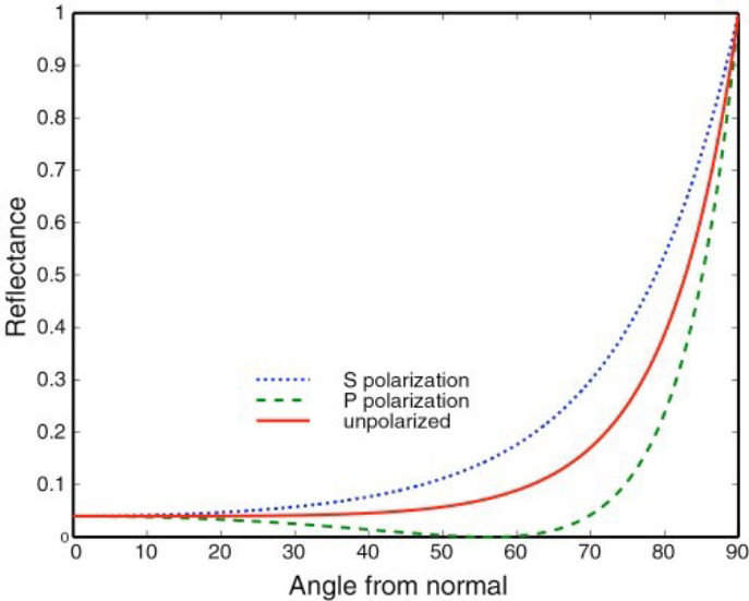
Reflectance varies with the angle of incidence (and light polarization), as illustrated in this example that shows how reflectance increases at grazing angles.

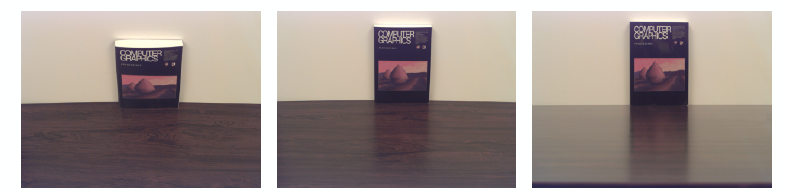
For dielectrics, such as water or glass, a significant amount of reflection is seen at grazing angles.

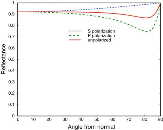
Similarly, with conductors, the trend is roughly the same. This is attributed to the polarization of light. However, understanding this in detail is beyond the scope of my current knowledge level and won’t be discussed further.

To summarize, the Fresnel term dictates: How much energy will be reflected!

More precisely, the Fresnel effect describes the relationship between the proportions of reflected and refracted light with respect to the viewing angle. This means that as the angle between the observation direction and the normal increases, the proportion of reflected light also increases.

In rendering, Schlick’s approximation is utilized to closely mimic the real Fresnel phenomenon:

F_{Schlick}(h, v, F_0) = F_{0} + (1- F_{0})(1 - h \cdot v)^5

F(0) = \frac{n_1-n_2}{n_{1}+n_2}^2

While I still don’t comprehend the rationale behind the fifth power, I understand its fundamental implication. Here, F0 acts like a base reflection; at an angle of zero, the reflectance is just F0. As the angle of incidence increases, the Fresnel term gradually increases.

We predefine a small F0 to represent the F0 of non-metallic materials. Then, a “metalness” parameter is assigned to the material: - If the metalness is 0, F0 takes the predefined value. - If the metalness is 1, it takes on the color of the metal itself. - In other cases, it is linearly interpolated. The unique characteristics of metallic surfaces, compared to dielectric surfaces, have led to the concept of the metalness workflow. This means we need an additional parameter called “metalness” to help describe the material’s surface as either metallic or non-metallic.

// Fresnerl term with scalar optimization  
vec3 F_Schlick(float VdotH, vec3 f0)  
{  
    float f = pow(1.f - VdotH, 5.f);  
    return f0 + (1.f - f0) * f;  
}

vec3 F0 = (1 - u_Roughness) * vec3(DIELECTRIC) + u_Roughness * vec3(material.baseColor);  

// F -- Fresnerl term with scalar optimization  
vec3 F = F_Schlick(VdotH, F0);

Normal Distribution Function (NDF)

The NDF (Normal Distribution Function) in the context of BRDFs (Bidirectional Reflectance Distribution Functions) is unrelated to normal distributions in statistics. Here, “normal” refers to the normals (or perpendicular vectors) of the microfacets on a surface. The NDF term signifies the distribution of these microfacet normals.

The following image provides a visual representation of this concept: 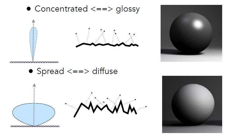For smoother surfaces, the reflected light tends to be more concentrated, producing a “glossy” or mirror-like reflection. On the other hand, rougher surfaces scatter light in various directions, giving a more “diffuse” appearance.

There are multiple models proposed to depict this phenomenon, such as the Beckmann and GGX models. Lingqi Yan has also contributed with improvements to these models in 2014, 2016, and 2018.

Here’s a comparison from Terragen showcasing the differences:

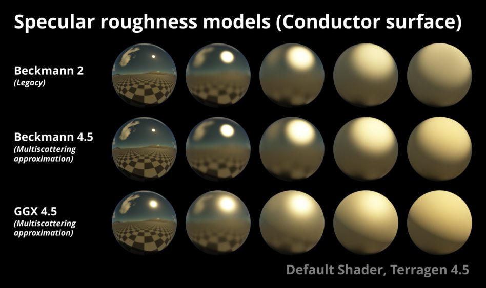
Presently, the GGX model (or Trowbridge-Reitz) [Walter et al. 2007], continues to dominate the industry, characterized by its distinctive long tail:

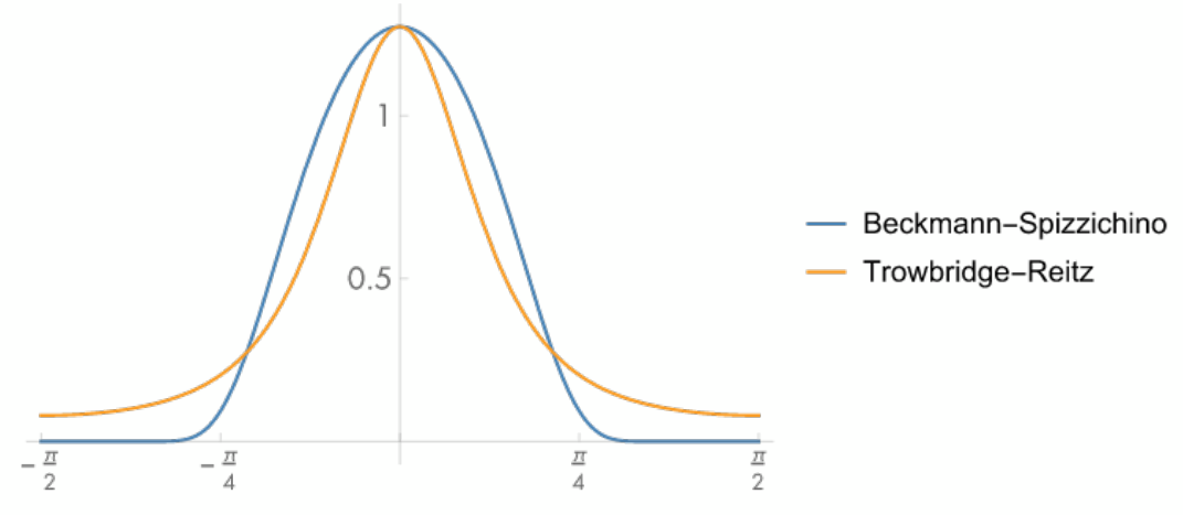
When comparing the distribution functions of the Beckmann-Spizzichino and GGX models, the Beckmann curve exhibits a more pronounced peak that decays rapidly. In contrast, the GGX curve has a broader but lower peak that tapers off gradually. This trait allows GGX to better approximate a broader range of real-world materials, particularly those with rough surfaces, enhancing its popularity.

The mathematical formulation for GGX is:

NDF_{GGX}(n, h, \alpha) = \frac{\alpha^2}{\pi({(n \cdot h) ^ {2} (\alpha^{2}-1) +1})^2}

The rationale behind using the half-vector is to measure the similarity between the normals of the microfacets and the normal at the intersection point.

It’s straightforward to incorporate this function into a shader:

// Normal Distribution Function using GGX Distribution  
float D_GGX(float NdotH, float roughness)  
{  
    float a2 = roughness * roughness;  
    float f = (NdotH * NdotH) * (a2 - 1.f) + 1.f;  
    return a2 / (PI * f * f);  
}

Shown below is the render result solely using the D term.

Shadowing-Masking Term (Geometry Term)

To address the issue of self-occlusion on microfacets, particularly at grazing angles, we need to account for how microfacets block or occlude each other. This phenomenon, known as self-occlusion, can be visualized as shadowing or masking, depending on whether the occlusion is viewed from the light source or the camera, respectively.

The following images offer a visual representation of this effect: From the light’s perspective, occlusion is termed as shadowing, and when viewed from the camera, it’s referred to as masking.

Given this self-occlusion, there’s an inherent potential for darkening. This is the crux behind the need for such a term in the BRDF.

This self-occlusion term is influenced by the angle between the camera and the intersection point. At near-perpendicular angles, the term has minimal effect since occlusion is unlikely. However, at significant grazing angles, the occlusion becomes more pronounced.

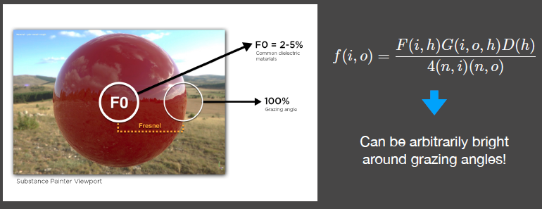
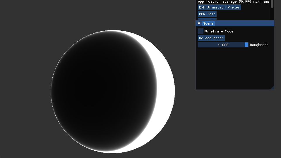
Consider a sphere, for instance. Without the G (geometry) term, if we assume the incident light comes from the camera’s position, the side with a grazing angle will approach 100%. This makes the denominator of the Cook-Torrance equation tend towards zero, resulting in a massive energy spike in light calculations. This can cause brightness to escalate arbitrarily around grazing angles.

The displayed rendered result illustrates the SpecularBRDF without the G term. The effect becomes markedly evident when the roughness increases.

A popular shadowing-masking term is the Smith shadowing-masking term. This term, derived from statistical assumptions, depicts the nature of self-occlusion. It can decouple shadowing from masking, which is mathematically represented as:

G(l, v, h) = G_{GGX}(l,h) \cdot G_{GGX}(v,h)

Where,

G_{GGX}(v, h) = \frac{n \cdot v }{(n \cdot v)(1-k) + k}

k = \frac{(\alpha + 1) ^2}{8}

From the following curve:

It’s evident that when light strikes vertically, there’s virtually no self-occlusion, hence the G term is almost inconsequential. Conversely, at high grazing angles, the G term undergoes significant variations, leading to a dramatic reduction in the overall BRDF value.

This can be seamlessly integrated into the shader with the following code:

// Geometry Term: Geometry masking/shadowing due to microfacets  
float GGX(float NdotV, float k)  
{  
    return NdotV / (NdotV * (1.f-k) + k);  
}  

float G_Smith(float NdotV, float NdotL, float roughness)  
{  
    float k = pow(roughness + 1.f, 2.f) /8.f;  
    return GGX(NdotL, k) * GGX(NdotV, k);  
}